Live-Casino & Sportwetten – WillBet bringt deutschen Nervenkitzel!
1999 hätte es gewiss niemand für möglich gehalten, welche Verbreitung heute kostenlose Browsergames finden. Damals gab es lediglich ein paar enthusiastische Hobby-Programmierer, die kostenlose Browserspiele in liebevoller Arbeit entwickelt und weiterentwickelt haben. Solche Games zu spielen, wurde eher belächelt. Besonders gute Onlinespiele ohne Download, heute ganz eindeutig mit an der Spitze der Beliebtheit, wurden kaum beachtet und nur von wenigen Spielern gespielt. Die einfache Grafik und die leicht zu erfassenden Spielprinzipien hielt man für amateurhaft - aber genau das ist es, was für Online Games heute, im Zeitalter von Web 2.0 und immer mehr und immer bedeutungsvolleren sozialen Netzwerken, den Durchbruch bedeutet hat.
Inzwischen sind
Browsergames in Deutschland, was das Internet und Social Media betrifft, der Trend schlechthin. Millionen von Usern nutzen sie, und jeden Monat werden es mehr, die sich auf unzählige verschiedene Titel stürzen, die auf dem Markt sind.
Live-Casino & Sportwetten – WillBet bringt deutschen Nervenkitzel!
Warum sind eigentlich so viele Browser Games kostenlos? Ganz einfach - auf diese Weise ist der Reiz besonders groß, sich einem Spiel anzuschließen; der Einstieg wird barrierefrei. So kommen sehr schnell unzählige Spieler für die verschiedenen Onlinespiele zusammen, was wiederum den Reiz erhöht, sie zu spielen, denn je mehr Gegner - oder Verbündete -, desto mehr Abenteuer und Spaß am Spiel. Das wissen natürlich auch die Spiele-Hersteller. Deshalb entstehen in den Entwicklerstudios so viele Browser Spiele für die Internutzer, die meist sehr schnell eine hohe Spielerzahl erreichen. Social Media wie Facebook.com tragen dabei sehr viel dazu bei, den Bekanntheitsgrad der beliebten Spiele zu verbessern und diese im Internet zu verbreiten.
Aber natürlich machen die Entwickler das nicht ganz uneigennützig; sie haben da schon so ihre Hintergedanken. Oft werden bei grundsätzlich kostenlosen Spielen, für die man einfach nur einen Account anlegen muss, mithilfe von sonst verschlossenen Zusatzleistungen Einnahmen erzielt - und das ist ja auch erlaubt, zumal man dabei zu nichts verpflichtet ist. Das ist das gleiche wie im Casino Spiele Bereich, wo fast alle Spiele kostenlos gespielt werden können, dem Spieler aber frei steht, auch um echtes Geld spielen zu können. Deshalb haben wir in diesem Portal die besten Browsergames, ob Warthunder, Die Siedler, Legends oder auch Automatenspiele - alle aus dem deutschsprachigen Sektor natürlich - zusammengesucht und stellen sie übersichtlich den Usern dar. Schließlich wollen wir alle, dass gratis Internetspiele nicht nur sind, sondern dies auch bleiben! Das größte deutsche Portal für kostenlose Spiele aus dem Gambling Bereich, das ausschließlich mit Spielgeld gespielt werden kann, ist das Spiele Portal jackpot.de. Wer noch keine Erfahrung mit einem Spielcasino ohne deutsche Lizenz gemacht hat, kann dort beliebte Slot-Games wie Big Bass Bonanza, Book of Inferno, Ghost Slider, Sizzling Hot & Co. ohne Risiko spielen. Generell kann man jedes Spiel was im Browser gespielt werden kann, als Browsergame bezeichnen. Dabei ist es egal, ob es ein einfaches Roulette Spiel ist oder die neueste Version von Sudoku auf einem HTML5 Spiele Portal ist. Immer wenn das Game im Browser startet ist es ein Browsergame.
Live-Casino & Sportwetten – WillBet bringt deutschen Nervenkitzel!
Einige der User, die regelmäßig Browsergames spielen, verschaffen sich über den Erwerb käuflicher Zusatzinhalte - spezielle Rüstungen oder Waffen, virtuelles Geld und anderes - Vorteile für den Spielerrang. Darüber erwirtschaften die Unternehmen, die Browserspiele ins Netz bringen, ihre Gewinne, die es ihnen möglich machen, auch in Zukunft gratis Spiele zu entwickeln und zu verbreiten. Natürlich gilt dies nur für die Browsergames mit unternehmerischem Hintergrund. Die Browserspiele, die von Freizeitprogrammierern entwickelt werden, denen das Lob der Community genügend Bezahlung ist, kommen ohne solche Features aus. Allerdings sind unter diesen Games, auch wenn sie durchaus spielenswerte und hochwertige 3D Browsergames sind, nur selten echte Blockbuster zu finden. Was nichts daran ändert, dass eine große Fangemeinschaft ihnen weiterhin die Treue hält.
Live-Casino & Sportwetten – WillBet bringt deutschen Nervenkitzel!
 In einer Zeit, in der es eine regelrechte Schwemme für Onlinespiele gibt, ist es umso wichtiger, die richtige Auswahl zu treffen und sich für das Spiel zu entscheiden, an dem man auch Spaß und Freude hat. Das wird häufig dadurch erschwert, dass man bei vielen dieser Online Spiele erst später erfährt, worum es eigentlich im Einzelnen geht, wenn man sich bereits angemeldet und einen Account erstellt hat. Umso wichtiger ist eine Webseite wie diese, auf der die verschiedensten Spiele vor einer Anmeldung vorgestellt werden, und zwar nach Genres unterteilt. Das macht die Auswahl leicht - oder doch zumindest leichter. Ganz sorgfältig, ausführlich und im Detail, mit Bildern und Videos, gehen wir auf Onlinespiele ein. Auch die Ranglisten, die es bei uns gibt, geben dem noch unentschlossenen User einen guten Einblick, was ihn in einem Spiel erwartet und ob sich die Anmeldung empfiehlt. Dabei lohnt es sich, immer mal wieder bei uns vorbeizuschauen. Denn ständig kommen neue Browsergames ohne Anmeldung auf den Markt. Wir bemühen uns, diese jeweils so schnell wie möglich mit einem umfassenden Testbericht vorzustellen. Damit machen wir besonders den ambitionierten Spielern den Einstieg leicht, die keine Lust haben, sich auf überfüllten Servern mit zahlreichen starken Gegnern herumzutreiben, sondern gleich ihren Spaß haben wollen. Bei uns können sie ihre Internetspiele ohne diesen Druck genießen.


 Immer ausgeklügeltere Endgeräte haben uns das mobile Internet gebracht, und diese modernen Internet-Technologien haben entscheidend dazu beigetragen, dass wir jederzeit und überall online gehen können. Diese Entwicklung hatte, neben dem wirtschaftlichen Nutzen und der Vereinfachung geschäftlicher Vorgänge, nicht zuletzt auch der Flexibilisierung des Arbeitsplatzes, auch für das Privatleben vieler Menschen seine positiven Folgen. Fast jeder hat schon mal ein typisches Browsergame gratis gespielt, und viele spielen sogar regelmäßig in ihrer Freizeit, mal nur für ein Break, mal als leidenschaftliches Hobby. Entsprechend wurden auch immer mehr Browserspiele entwickelt, sodass mittlerweile die Auswahl mehr und mehr schwer fällt. Deshalb haben wir in diesem Portal die besten Online Games - alle aus dem deutschsprachigen Sektor natürlich - zusammengesucht und stellen sie übersichtlich den Usern dar. Dabei haben wir die Spiele nach verschiedenen Genres geordnet, sodass jeder schnell für sich das passende Game findet. Und falls man einmal nicht weiter weiß, helfen die User sich in Foren und Chats gegenseitig mit Tipps und Tricks zu jedem Titel. Gerade "Newbies", also Neulinge, finden so schnell Hilfe für beliebte Onlinespiele und finden in der Gemeinschaft sogar gleich noch soziale Kontakte. Damit können sie sich zum Beispiel auch schnell selbst an komplizierte
  Mars Tomorrow
 New World Empires
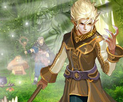
 Forge of Empires
 Zoo 2: Animal Park
 World of Tanks
 Pirates of the Caribbean: Tides of War
 Dinosaur Park
 My Little Farmies
 Travian
 War Thunder


 In einer Zeit, in der es eine regelrechte Schwemme für Onlinespiele gibt, ist es umso wichtiger, die richtige Auswahl zu treffen und sich für das Spiel zu entscheiden, an dem man auch Spaß und Freude hat. Das wird häufig dadurch erschwert, dass man bei vielen dieser Online Spiele erst später erfährt, worum es eigentlich im Einzelnen geht, wenn man sich bereits angemeldet und einen Account erstellt hat. Umso wichtiger ist eine Webseite wie diese, auf der die verschiedensten Spiele vor einer Anmeldung vorgestellt werden, und zwar nach Genres unterteilt. Das macht die Auswahl leicht - oder doch zumindest leichter. Ganz sorgfältig, ausführlich und im Detail, mit Bildern und Videos, gehen wir auf Onlinespiele ein. Auch die Ranglisten, die es bei uns gibt, geben dem noch unentschlossenen User einen guten Einblick, was ihn in einem Spiel erwartet und ob sich die Anmeldung empfiehlt. Dabei lohnt es sich, immer mal wieder bei uns vorbeizuschauen. Denn ständig kommen neue Browsergames ohne Anmeldung auf den Markt. Wir bemühen uns, diese jeweils so schnell wie möglich mit einem umfassenden Testbericht vorzustellen. Damit machen wir besonders den ambitionierten Spielern den Einstieg leicht, die keine Lust haben, sich auf überfüllten Servern mit zahlreichen starken Gegnern herumzutreiben, sondern gleich ihren Spaß haben wollen. Bei uns können sie ihre Internetspiele ohne diesen Druck genießen.